By Alex White FIA C.Act, Global Head of Quantitative Modelling at Gallagher
This is probably provable in closed-form by a better mathematician than me, but I can show it with simulations. Suppose we have a portfolio of 10 stocks, each 50% correlated with each other, and each with a geometric 8% return and 30% (ln) volatility. We run it for 10 years, with no rebalancing.
If we never sell a stock, and just take the final value, the IRR and returns are, by definition, identical (at 10.4%) – so far so good. But what happens if we start selling part way through?
Suppose the manager sells any individual stock that outperforms an N x return each year. For example, if a stock in year 4 is worth more than 4 times its original value, then it gets sold.
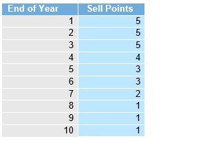
This is a sensible thing to do, at least within the assumptions of this simulation, as it limits concentration, and therefore reduces volatility, and so increases both diversification and geometric returns. In this example though, while hard to quantify precisely, we can cap the effect. The maximum benefits of rebalancing would be attained by full annual rebalancing, and we can estimate this by comparing the theoretical volatility of a fully rebalanced portfolio (22%) with the simulated, non-rebalanced portfolio (25%), and using exp(Vol^2/2) we know this effect is less than 0.8%. In all likelihood it’s materially less, as the residual portfolio after any sales would also be quite far from equal weighted. So, we might expect a boost of about half, or 40bps.
The IRRs, meanwhile, shoot up to 12.4%, meaning the IRRs are about 2 percentage points higher than the underlying returns, or 1.5% even allowing for some rebalancing advantage. And by construction, this isn’t from any skill in selection, this is just from the maths of IRRs. By getting paid early, the IRR looks higher, even though there was no way to keep that reinvestment rate.
Of course, it’s hard to know what the underlying volatility of a private asset really is, in any unsmoothed, economic sense. What’s easier is checking the sensitivity of this “IRR pickup” over returns. Fundamentally, the impact of volatility here is really how likely any stock is to breach a sale point. If we raise it to 40%, the returns are 12.3%[1] and the average IRR is 16.3%. At 50% volatility, these jump to 14.6% and 22.3%, a whopping 8% pickup in expected IRR over expected returns.
This isn’t an attack on private assets, which can and often do deliver outsized returns. This isn’t an attack on managers either. Many of the assumptions, such as the sale points, are arbitrary, and the results are not intuitive to interpret- the values we’re considering are the expected values of IRRs given the expected returns on the underlying assets. However, it highlights a mathematical quirk, which gives another reason to give pause when assessing an investment, and to not give too much weight to any spectacular historic IRRs.
[1] The reason a higher vol assumption drives a higher return is we assume the 8% is geometric, so it makes the arithmetic return per stock higher, and gives a larger pickup from diversification
|