By Alex White, FIA, Global Head of Quantitative Modelling at Gallagher
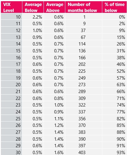
So we took different VIX levels and compared the average (ln excess) return for subsequent months (out of 435 total), conditional on whether the VIX was above or below each level. The long term average level has been 20.
VIX levels against next month’s returns- source Gallagher, Bloomberg, Refinitiv
This suggests that higher levels of VIX can predict higher subsequent returns. So should we all “buy the dip”?
Well, maybe. The risk is this all makes sense mathematically without the VIX having any extra information- when the VIX has spiked, that’s generally because equities have just fallen. So returns just after a big loss are higher than those from a larger sample that includes the big loss.
Perhaps the most informative insight comes from looking at absolute values of returns. While excess returns have been essentially uncorrelated month on month, their absolute values have been 20% autocorrelated, and initial VIX levels are almost 50% correlated with subsequent absolute moves. In other words, volatility shows a degree of short-term persistence. So spikes in the VIX can predict spikes in short term volatility. More underwhelming conclusions have probably been reached, but I can’t think of many.
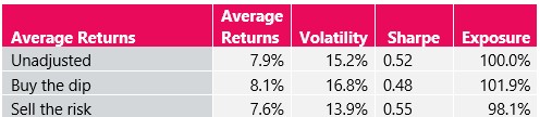
So what happens when you try to make it a trading algorithm? You wouldn’t have known, in 1990, that the average VIX level would be about 20[2], so we use rolling percentiles. We also allow 5 years to run to stabilise the levels, but this doesn’t materially change the outputs. We then add 20% exposure when the VIX is in the bottom 20% of rolling historical levels, and reduce by 20% when it’s in the top 20% (“Buy the dip”). We also add another strategy, “Sell the Risk”, which does the exact opposite.
Trading based on VIX levels - source Gallagher, Bloomberg, Refinitiv
This paints a more nuanced picture. Returns may be higher, but when VIX is elevated risk-adjusted returns are broadly worse (this is true even if we adjust the strategies so they give an overall average exposure of 100%). It also treats equities in isolation- but after a fall, portfolios are likely to be underweight equity. And the fall in Sharpe can be explained by the maths, as log returns don’t scale linearly.
So what should investors do in periods of heightened volatility? Well, broadly just keep calm, look for opportunities and dislocations, and trust their SAAs.
[1] An index of implied volatilities for options on the S&P500
[2] arguably this is less of an issue here than in other cases, such as what should P/E ratios be, because there are long-term equity series with long-term volatilities, and we know equities have fat-tails, so a rational investor in 1990 would likely have guessed a number that was something a bit bigger than 15%. But whether the “right” number was 16 or 25 would have been less knowable.
|