By Alex White, Head of ALM Research at Redington
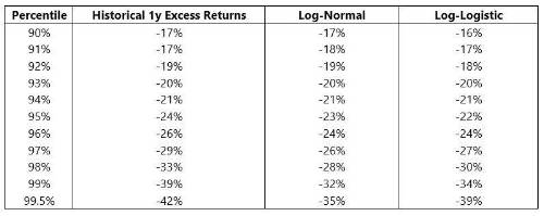
As a general guide to building a model, it makes sense to start with the largest components with the most data. Using Shiller’s data, we can track US equity excess returns back to 1870 and compare these to what we’d expect from a log-normal and a log-logistic distribution (which ends up looking somewhat like a fat-tailed normal distribution). The famous fat tails in equity distributions only really appear beyond the 5% tail.

This can be interpreted as evidence for either approach. On the one hand, if historic returns are more straightforward up to around the 95th percentile mark, then you can have far more confidence in that figure. On the other hand, if the extreme tail has experienced far more dramatic moves, you might want a risk metric that tracks it.
It’s worth stepping back and thinking about how this data emerges. If I have 150 years of equity returns, I should expect around 7 or 8 95th percentile moves – especially since the distribution is not overly dramatic at that point. Therefore, I can be fairly confident that I have a sensible answer. However, for the 99th percentile, I should only expect 1 or 2 cases.
That’s all true, but not massively helpful. Instead, can we translate this uncertainty into something easier to understand?
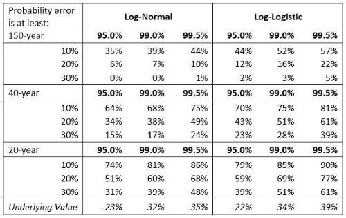
In the table below, we simulated 10,000 random historic 150-year periods, assuming either a log-normal or a log-logistic distribution.
This shows how likely it is that the value observed over any given 150-year period was more than a given percentage error away from the underlying ‘true’ value. We express these as absolute (not log) returns and run them for 40-year and 20-year time horizons.
For the log-normal distribution, the increased uncertainty is largely offset by the increased range (as the allowed error is proportional to shock size). However, as soon as the distribution has fat tails, the tails become less predictable. This analysis assumes equities follow a simple distribution and that the parameters we happen to have observed are the true underlying ones, so this will understate the risk of being wrong. Even so, there’s still a 5% chance that the historical 95th percentile is more than 30% off the true value. And this is with equities; for many risk factors we have much shorter histories. Even with these generous assumptions, with a 20-year history (for example), it’s more likely than not that the realised 99th percentile is more than 30% out.
Which means that, when you get into the tail, you really don’t know how extreme things will be and so you’re having to extrapolate a distribution out anyway. Hence, while the extreme tail may be a useful secondary risk metric, for most cases it makes sense to compromise and use a less extreme, less uncertain part of the tail as the main risk metric.

|

