By Alex White, Head of ALM Research at Redington
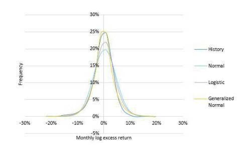
The logistic distribution has kurtosis of 1.2, the normal distribution has zero, and the history has kurtosis just under ten. Without going into too much of the detail, we can see graphically that the generalised normal distribution, though needing a third parameter, is a better fit to the history.

We show the distribution parameterised by maximum likelihood estimation (MLE), and it’s optically a pretty good model. However, there are a couple of important nuances worth knowing before using it anywhere.
Firstly, the kurtosis is surprisingly low, at 2.5. This is from a very flexible distribution, but it has to fit the whole shape. It turns out the best fit is still substantially less fat-tailed. The second is a quirk that the MLE can pick the location parameter (effectively the expected return) closer to the median than mean, which happens here. It’s not immediately a huge difference- the median is 0.6% while the mean is 0.4%- but compounded over a year it’s quite meaningful.
This starts to be much more pronounced when we compound up, and look at the resultant distribution over a year. To give the more complex distribution the best chance possible, we include the historical autocorrelation of 24% between subsequent months. Based on 12 months, each with 10,000 simulations, we get a distribution with a volatility of 16%, a kurtosis of 0.2, a skew of -1%, and a mean of 7.5%. The annual VaR95 is 19%. For context, the history has a mean of 4.5% and an annualised monthly volatility of 14%, or a volatility of annual returns of 19%. Fitting a normal distribution would give a VaR95 of 19%, as against a historical figure of 23%.
So far so good, but let’s think about what that entails when using either approach for a model. Which is a better choice, and what adjustments you might make, will depend on what purpose it’s being used for. But there are good reasons to challenge the more complex model. Firstly, it has a mean noticeably higher than that justified by the 150y history, and with negligible skew and kurtosis it looks a lot like a normal distribution with a higher mean and higher standard deviation. That’s potentially very problematic in any scenario where the upside is important, as it will dramatically overstate the upside, especially when converted from log returns.
Obviously there are better models than a simply calibrated normal distribution, but for many goals the generalised normal distribution, fit by MLE to monthly returns, may well ironically be worse.
Now, this is not quite an example of the central limit theorem (CLT), but it’s similar, and much easier to make puns on CLT than on kurtosis. That aside, there is a serious point, which is that adding complexity- and even adding apparent accuracy- to a model is not necessarily an improvement. We know in finance that the underlying behaviour is extremely complex and to some extent influenced by which models are commonly used to proxy it. We can’t capture precise behaviour so we’re merely trying to get sensible answers to specific questions. And that may mean being pragmatic rather than purist about the models.
|


