By Alex White, Head of ALM, Redington
For example, while year-on-year data is largely uncorrelated (c1%), monthly data is 26% autocorrelated. So, a bad month is likely to be followed by another bad month. This is fundamental to trend investing, and is why even simple trend strategies can make money.
For daily data the effects are stronger, which makes sense. If there’s new information, that should impact the price as soon as it’s known (even if it takes a while longer to feel the full impact, some of it happens upfront). In the extreme case, in almost all femto-seconds nothing happens, and in a miniscule proportion of them a trade occurs and the price moves. The volatility would be almost zero, yet the tail risk would still be there. If you are a long-term investor though, you probably care more about annual or multi-annual returns than daily (or even shorter-term) returns, and the problem is a lot smaller at longer horizons.
The flipside of looking at longer horizons is that you have less data. If you care about annual returns, 150 years of data means 150 independent points, as against c40,000 daily data points. This means that even at the 5th percentile, any historical VaR95 is only based off 7-8 genuinely different data points, and anything beyond the 0.7th percentile is extrapolated. While this can be somewhat mitigated by using rolling data, this does not create more data, it effectively just smooths the existing set. This means it is difficult to have confidence in any calibration of tail risk for longer horizons.
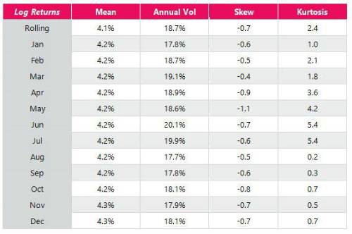
Another issue is that the higher moments are unstable, even over 150 years. When looking at annual data, which month you start at makes an enormous difference, as seen in the table below. For example, the (excess) kurtosis varies from 0 (August-August data) to 5 (July-July). This means calibrating a model to historical kurtosis is somewhat fraught.
So where does this leave us? The conclusion may be somewhat uninspiring and unoriginal, but the further into the tail you go, the less you should trust any model. The one caveat to this point is that your personal intuition is just another model. It has all the same problems as any quantitative model, and it’s hard to justify that our brains would have a particularly good mechanism for modelling equity tail risk. When you go deep into the tail, you just have to accept a greater degree of uncertainty.
The table below is based on US equity excess returns from 1870 using data from Professor Shiller and the S&P 500.
|